CSE168 Final Project: Chess in the Morning
Siddhartha Saha (ssaha at ucsd dot edu)
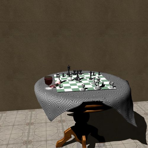
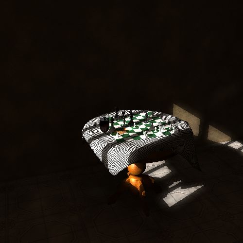
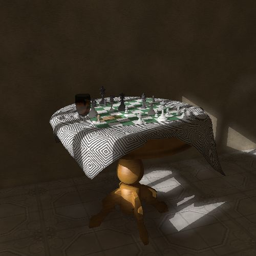
Let me present the final pictures first.
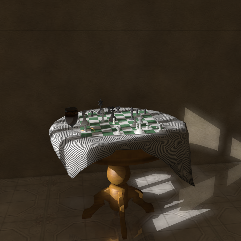
(153636 Triangles, Rendered at 800×800 with 4×4 AA, which took
11838.964 sec in my laptop, 1.6Mhz Pentium M, 768MB RAM)
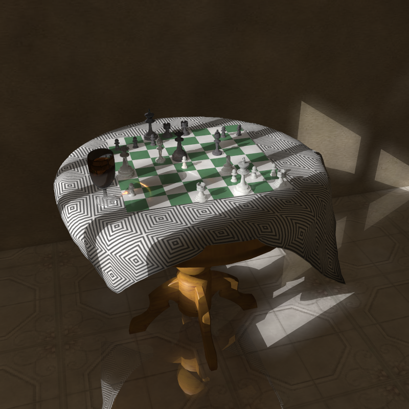
(153636 Triangles, Rendered at 800×800, with 4×4 AA, took 17919.813 sec in my lab PC (Athlon Xp 2200+, 512MB)
Now for the descriptive part.
Implementation:
A basic ray tracer was used. The code of the ray tracer was based on the skeletal code and the scripting language that was given to the class by our T.A., Craig Donner. Even though the final version of the ray tracer that was used the render the image above was nowhere close to the original code, I was too lazy to change the name of the ray tracer, and kept it throughout asmiro.
Some of the things that the ray tracer (miro) supported:
-
Global Illumination with photon mapping
-
Soft Shadows, Area/Directional/Point/Sphere lights, with MC sampling used to generate soft shadows.
-
A basic scene definition language (Credit goes to Craig)
-
Anti-aliasing using super-sampling
-
Bump mapping, texturing. I did not implement procedural texture though.
-
It can import Alias Wavefront .obj files, with materials from .mtl file as well as PLY file.
-
As acceleration structure, it has Uniform/Hierarchical/Adaptive grids, as well as a Bounding Volume Hierarchy
-
Support for Fresnel Refraction.
etc.
But
due to the simplicity of the model that I finally managed to render, some of these features were not used in the final rendering.
The Path Taken:
I spent a lot of time coding than doing the actual modeling and rendering. The basic ray tracer was working pretty well up-to the implementation of Adaptive Grids as an acceleration structure (till the end of the third assignment). After that I added texture support, a module to load Alias Wavefront object models with proper material support. incorporated global illumination and caustic rendering using path tracing, (which was way too slow by the way), photon mapping (I love this approach), bump mapping. I used the famous Cornell Box to test some of the approaches. Here are some random images:
 |
| A very high polygon image of a Chinese Dragon (From The Stanford 3D Scanning Repository). This is one image from the very early stage of the Ray Tracer, and at some point in time I was also thinking of rendering this as my final image with subsurface scattering, but that plan never materialized. (I had to write a PLY format reader for it) |
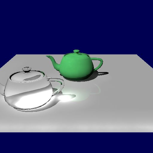 |
| This is an image of a caustic from a solid glass teapot. This is also one of the early images while implementing the photon maps. |
 |
| My first somewhat successful rendering of the Cornell Box. This was done without using photon maps. |
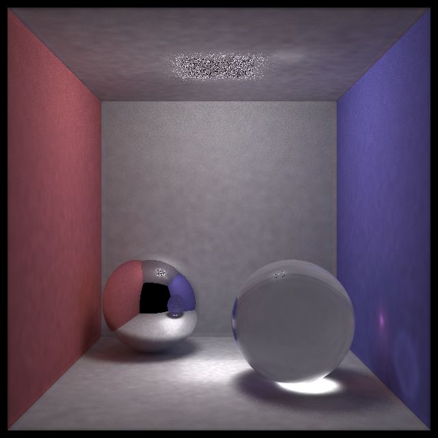 . . |
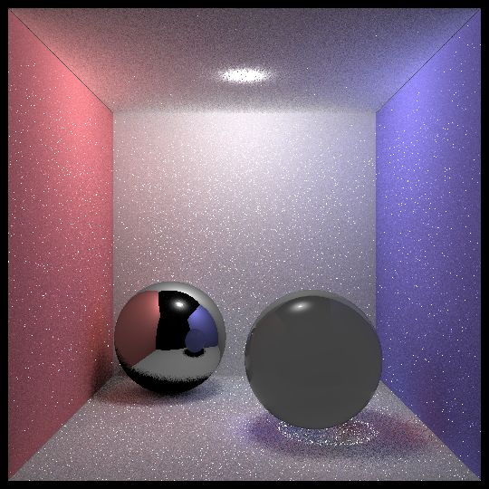
| Cornell Box rendering with photon maps. |
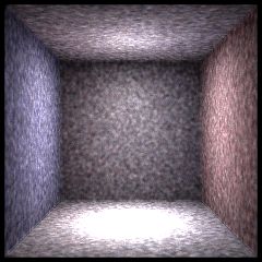 |
| A direct visualization of a indirect illumination using (rather coarse) photon maps (with the mirror and glass balls omitted). |
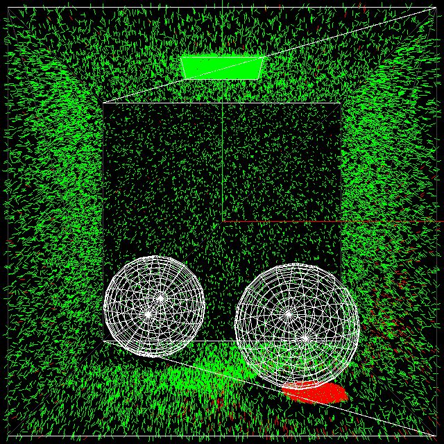 |
| The photons in the Cornell box. The green ones are global photons, and the red ones are caustic photons. |
What to Render?
I was baffled by this question for quite a long time, and I was always postponing my decision by making further changes to the ray tracer. Which, in retrospect, was a mistake, since, at the end I had a ray tracer at my disposal, but with nothing to render. I toyed with a few ideas. The first one being a moonlit beach. But the modeling was rather difficult, and I realized with horrors that I am a terrible modeler, and modeling is not my forte . Then I thought of rendering some building the models for which could potentially be picked from the internet. But this turned out to be a futile effort. In the limited time that I had, I could not find any good architectural marvel that I could render as my final project. The deadline was approaching, and finally it occurred to me that a lonely chessboard with a wine glass beside a window with morning sunshine seeping in that can be modeled and rendered pretty quickly. It would have been nice if I could implement the participating media, but I just ran out of time after the modeling got over.
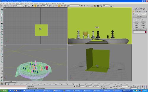
The Modeling:
I mostly used 3D Studio Max, a little Maya and some other format conversion softwares to model my scene. The first and foremost thing that I did was to model the chessboard and the chess pieces. Which took much longer than I expected. I got the table and few chessmen pieces off the internet, as they were too complex for me. I also had a glass of wine placed at the table, the following two pictures shows those two images
|
|
|
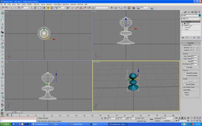
I tried to model the chessmen pieces by rotating a |
|
|
|
Another snapshot of building the model. |
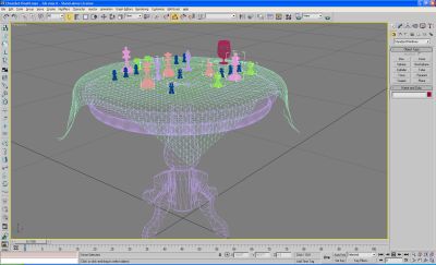
Modeling the tablecloth were really complex. But finally I
managed to do it with 3D Studio. I used the reactor in 3D Studio to model
the table cloth. The following two pictures show the tablecloth and the final
model that I managed to build.
|
|
|
The table, table cloth, the chessmen and the glass |
|
|
|
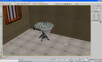
The final model as seen in in the modeler. |
Building the Final Image:
Once I got the modeling done, I started rendering the model. The initial renders were without the photon maps, just to test if everything was going all right. I tried many different variations over here, like deciding on direction of the light, where to put the table in reference to the window. Experimented with some details. Tried to add a bump map to the table cloth to make the threads visible, but the effect was not so nice, so I dropped the idea. I used an adaptive grid as an acceleration structure, which works really well. The final model had over 150 thousands of triangles.
|
|
|
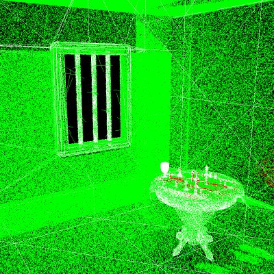
The final wire mesh model rendered. The faint yellow (not quite visible) boxes are the bounding volume hierarchy of the adaptive grid. |

Here are some initial renderings of the image:
 |
| This is the first rendering of the image. It was lit by a directional light (Simulating the sun). The complete scene was open to lighting, the window and other walls were removed in this image. Only the floor and the visible wall was left intact. |
 |
| This is the rendering of the scene with the walls and window in place, and with the photon mapping turned on. It seems a bit dark, and I had to tweak with the parameters of the light to get the correct brightness. Moreover, I did not use tone mapping in this image. |
 |
| The image with some lighting adjustment and tone mapping. |
 |
| This is the view of the photon map from before the final rendering. I used about 3,000,000 global photons, and 50,000 caustic photons to render the final image. |
… and finally this produced the pictures those are shown in the beginning of the page. It really came out pretty nice.
Acknowledgements:
Two resources that I found particularly useful were (1) Henrik’s course notes of “A Practical Guide to Global Illumination using Photon Mapping, SIGGRAPH 2002 Course 43” and (2) “Global Illumination Compendium” by Philip Dutré.